dynpy tutorial
Introduction
dynpy is a package for defining and running dynamical systems in Python. The goal is to support a wide-variety of dynamical systems, both continuous and discrete time as well as continuous and discrete state.
dynpy is organized into a hierarchy of classes, with each class representing a different kind of dynamical system. The base classes are defined in dynpy.dynsys - Base module for dynamical systems. Some definitions used for creating sample systems in this tutorial are defined in dynpy.sample_nets - Module with sample networks and dynamical systems.
Example: Boolean Networks
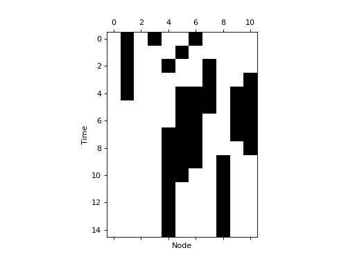
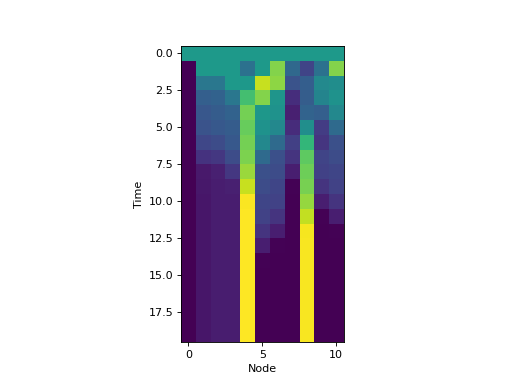
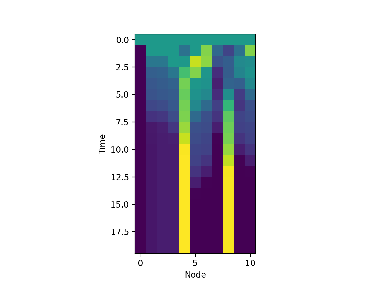
Boolean network are a type of discrete-state, discrete-time dynamical system. Each node updates itself as a Boolean function of other nodes (its ‘inputs’).
dynpy.bn - Boolean network module implement Boolean network dynamical systems. For example, we can use it to compute the space time diagram of the 11-node yeast cell-cycle network, as described in: Li et al, The yeast cell-cycle network is robustly designed, PNAS, 2004.
import matplotlib.pyplot as plt
import numpy as np
import dynpy

bn = dynpy.bn.BooleanNetwork(rules=dynpy.sample_nets.budding_yeast_bn)

initState = np.zeros(bn.num_vars, 'uint8')
initState[ [1,3,6] ] = 1
plt.spy(bn.get_trajectory(start_state=initState, max_time=15))
plt.xlabel('Node')
plt.ylabel('Time')
(Source code, png, hires.png, pdf)

We can also get the network’s attractors, by doing:
>>> import dynpy
>>> bn = dynpy.bn.BooleanNetwork(rules=dynpy.sample_nets.budding_yeast_bn)
>>> atts, attbasins = bn.get_attractor_basins(sort=True)
>>> print(list(map(len, attbasins)))
[1764, 151, 109, 9, 7, 7, 1]
Or print them out using:
>>> import dynpy
>>> bn = dynpy.bn.BooleanNetwork(rules=dynpy.sample_nets.budding_yeast_bn)
>>> bn.print_attractor_basins()
* BASIN 1 : 1764 States
ATTRACTORS:
   Cln3    MBF    SBF Cln1,2   Sic1   Swi5  Cdc20 Clb5,6   Cdh1 Clb1,2   Mcm1
      0      0      0      0      1      0      0      0      1      0      0
--------------------------------------------------------------------------------
* BASIN 2 : 151 States
ATTRACTORS:
   Cln3    MBF    SBF Cln1,2   Sic1   Swi5  Cdc20 Clb5,6   Cdh1 Clb1,2   Mcm1
      0      0      1      1      0      0      0      0      0      0      0
--------------------------------------------------------------------------------
* BASIN 3 : 109 States
ATTRACTORS:
   Cln3    MBF    SBF Cln1,2   Sic1   Swi5  Cdc20 Clb5,6   Cdh1 Clb1,2   Mcm1
      0      1      0      0      1      0      0      0      1      0      0
--------------------------------------------------------------------------------
* BASIN 4 : 9 States
ATTRACTORS:
   Cln3    MBF    SBF Cln1,2   Sic1   Swi5  Cdc20 Clb5,6   Cdh1 Clb1,2   Mcm1
      0      0      0      0      1      0      0      0      0      0      0
--------------------------------------------------------------------------------
* BASIN 5 : 7 States
ATTRACTORS:
   Cln3    MBF    SBF Cln1,2   Sic1   Swi5  Cdc20 Clb5,6   Cdh1 Clb1,2   Mcm1
      0      0      0      0      0      0      0      0      0      0      0
--------------------------------------------------------------------------------
* BASIN 6 : 7 States
ATTRACTORS:
   Cln3    MBF    SBF Cln1,2   Sic1   Swi5  Cdc20 Clb5,6   Cdh1 Clb1,2   Mcm1
      0      1      0      0      1      0      0      0      0      0      0
--------------------------------------------------------------------------------
* BASIN 7 : 1 States
ATTRACTORS:
   Cln3    MBF    SBF Cln1,2   Sic1   Swi5  Cdc20 Clb5,6   Cdh1 Clb1,2   Mcm1
      0      0      0      0      0      0      0      0      1      0      0
--------------------------------------------------------------------------------
Cellular Automata
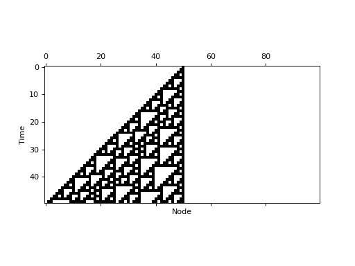
The cellular automata class dynpy.ca.CellularAutomaton is defined in
dynpy.ca - Cellular automata module. It is a subclass of dynpy.bn.BooleanNetwork.
It constructs a Boolean network with a lattice connectivity
topology and a homogenous update function. For example:
import matplotlib.pyplot as plt
import numpy as np
import dynpy

ca = dynpy.ca.CellularAutomaton(num_vars=100, num_neighbors=1, rule=110)

initState = np.zeros(ca.num_vars, 'uint8')
initState[int(ca.num_vars/2)] = 1
plt.spy(ca.get_trajectory(start_state=initState, max_time=50))
plt.xlabel('Node')
plt.ylabel('Time')
(Source code, png, hires.png, pdf)
Markov Chains
dynpy also implements Markov chains, or dynamical systems over distributions of
states. See the documentation for dynpy.markov.MarkovChain for more
details.
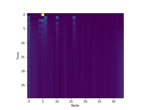
For example, here we use dynpy.graphdynamics - Module for implementing dynamical systems on graphs, which implements dynamics on
graphs, to instantiate a dynamical system representing the distribution
of a random walker on Zachary’s karate club network. Here,
dynpy.graphdynamics.RandomWalker is a subclass of
dynpy.markov.MarkovChain.
import matplotlib.pyplot as plt
import numpy as np
import dynpy

G = dynpy.sample_nets.karateclub_net
N = G.shape[0]
rw = dynpy.graphdynamics.RandomWalkerEnsemble(graph=G)

initState = np.zeros(N)
initState[ 5 ] = 1

trajectory = rw.get_trajectory(start_state=initState, max_time=30)
plt.imshow(trajectory, interpolation='none')
plt.xlabel('Node')
plt.ylabel('Time')
(Source code, png, hires.png, pdf)

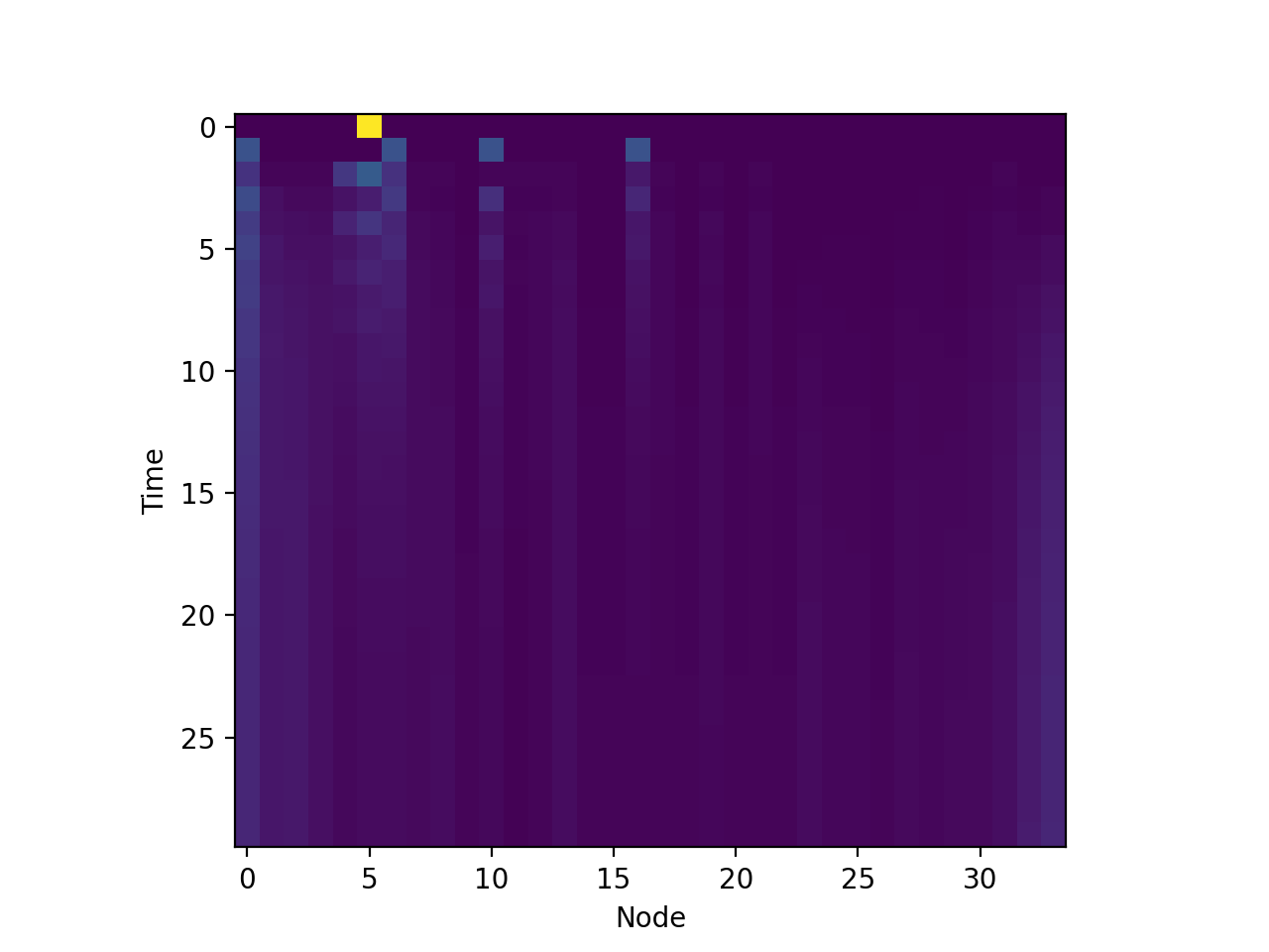
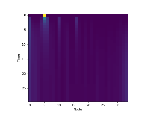
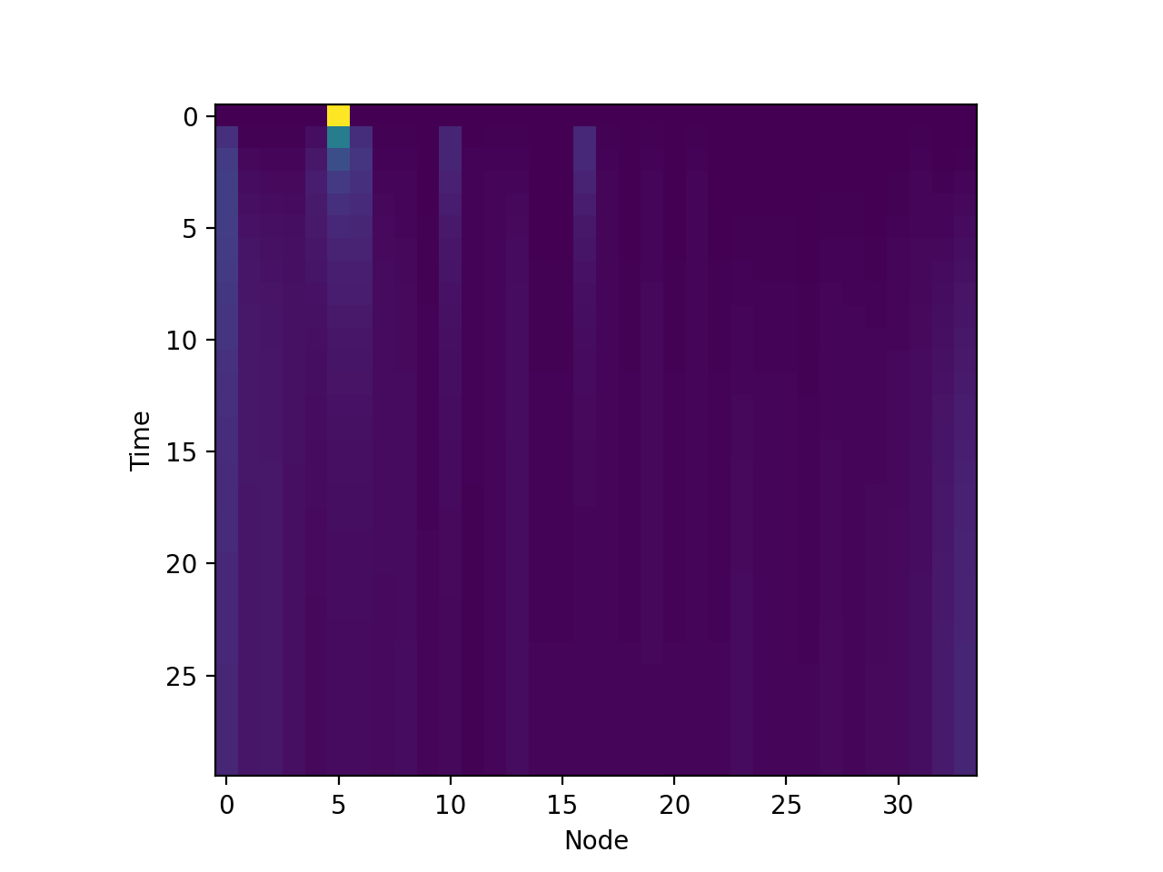
A Markov chain, like some other dynamical systems implemented by dynpy, can also
be run in continuous time (in this context, it is sometimes called a ‘master
equation’). This is specified by passing in the discrete_time=False option when
constructing the underlying dynamical system. Using the previous example:
import matplotlib.pyplot as plt
import numpy as np
import dynpy

G = dynpy.sample_nets.karateclub_net
N = G.shape[0]
rw = dynpy.graphdynamics.RandomWalkerEnsemble(graph=G, discrete_time=False)

initState = np.zeros(N)
initState[ 5 ] = 1

trajectory = rw.get_trajectory(start_state=initState, max_time=30)
plt.imshow(trajectory, interpolation='none')
plt.xlabel('Node')
plt.ylabel('Time')
(Source code, png, hires.png, pdf)

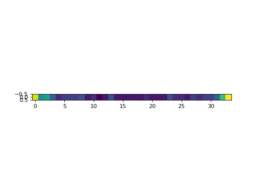
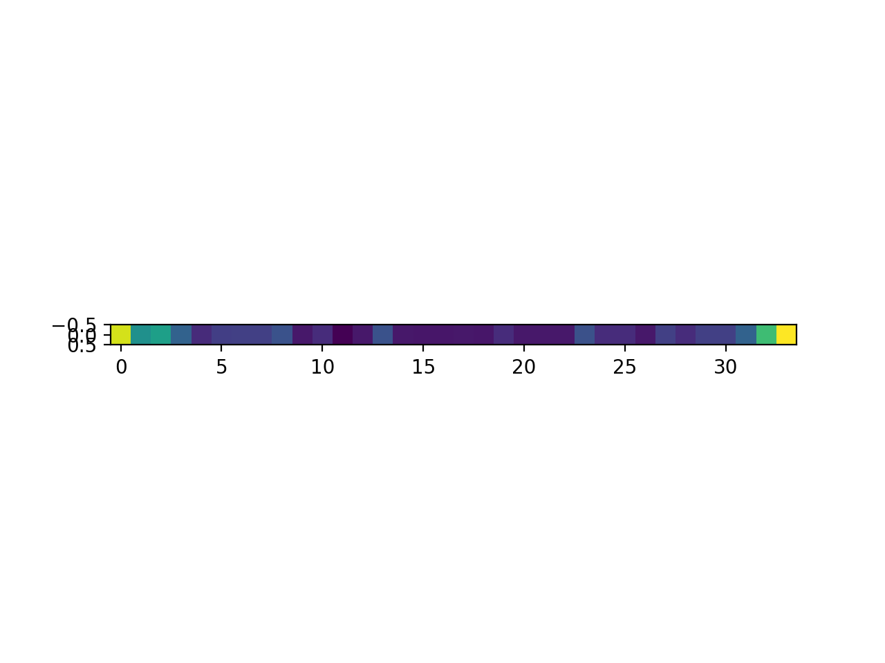
It is also possible to get the equilibrium distribution by calling
get_equilibrium_distribution(), which uses eigenspace decomposition:
import matplotlib.pyplot as plt
import numpy as np
import dynpy

kc = dynpy.sample_nets.karateclub_net
rw = dynpy.graphdynamics.RandomWalkerEnsemble(graph=kc, discrete_time=False)

eq_state = rw.get_equilibrium_distribution()
plt.imshow(np.atleast_2d(eq_state), interpolation='none')
(Source code, png, hires.png, pdf)

In fact, it is possible to turn any deterministic dynamical system into a Markov
chain by using the dynpy.markov.MarkovChain.from_deterministic_system() method.
For example, to create a dynamical system over a distribution of states of
the yeast-cell cycle Boolean network:
import matplotlib.pyplot as plt
import dynpy

bn = dynpy.bn.BooleanNetwork(rules=dynpy.sample_nets.budding_yeast_bn)
bnMC = dynpy.markov.MarkovChain.from_deterministic_system(bn)

# get distribution over states at various timepoints
t = bnMC.get_trajectory(start_state=bnMC.get_uniform_distribution(), max_time=20)

# project back from states onto activations of original nodes
bnProbs = t.dot(bn.get_ndx2state_mx())

# plot
plt.imshow(bnProbs, interpolation='none')
plt.xlabel('Node')
plt.ylabel('Time')
(Source code, png, hires.png, pdf)

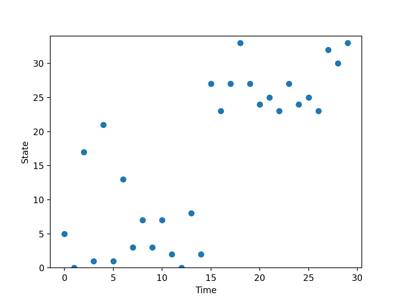
Stochastic Systems
Stochastic systems can also be implemented.
import matplotlib.pyplot as plt
import numpy as np
import dynpy

num_steps = 30
G = dynpy.sample_nets.karateclub_net
N = G.shape[0]
rw = dynpy.graphdynamics.RandomWalkerEnsemble(graph=G)
sampler = dynpy.markov.MarkovChainSampler(rw)

# Initialize with a single random walker on node id=5
trajectory = sampler.get_trajectory(start_state=5, max_time=num_steps)

plt.plot(np.arange(num_steps), trajectory, 'o')
plt.ylim([0, rw.num_states])
plt.xlabel('Time')
plt.ylabel('State')
(Source code, png, hires.png, pdf)
